Recap of Week 4

The topic covered for this week in the study was chapter 4 of the book Deep Learning for Coders on going deeper into computer vision with MNIST dataset to build a Digit Classifier.

I am jotting down some of topics covered during the session:

Pixels are the foundation of images.
Here we are using the MNIST dataset to explore Deep learning.
We are using dataset URLs.MNIST_SAMPLE, which is a sample of images of 3 and 7. There is another dataset the popular MNIST dataset which can be accessed via URLs.MNIST containing handwritten images from digits 0-9.
In computer ideally for easier computations we need everything in an array or in mathematic terms a symmetric matrix.
Aman during the session, asked how to classify an image of 3 and 7?
Lot of wonderful ideas were discussed on how to classify images in the discussion thread.
Like classifying number based on surface percentage of the coloured densities in the tensor of background to tell what percentage is covered by number to classify.
We decided to go with Pixel similarity, that is to find the average value for every pixel of images of 3s and 7s. Then the two group averages define what is the ideal 3 and ideal 7
what is the difference between tensor and array? > An array is a terminology in NumPy and tensor for PyTorch.
rank is the number of axes or dimensions in a tensor.
shape is the size of each axis of a tensor.
Now for our ML model, to distinguish between images of 3 and 7. With pixel similar what it does is:
Check by comparing our mean images of 3 and 7 obtained by stacking images.
Then you compare the new image(to predict) and find the difference between the mean of 3 and 7.
As Aman pointed out, when subtracting between two unlike quantities there is a possibility to cancel out.

So for calculating calculating difference with the predictions and correct value we used loss functions.
L1 loss is basically just calculating absolute difference between actual & predicted.
Another loss function calculates by finding the difference and then squaring(L2 loss- Root mean squared loss)
Major differences b/w Pytorch and Numpy framework are:

Pytorch works on GPU and Numpy is working on CPU
Pytorch can automatically calculate gradients & while numpy can’t do it

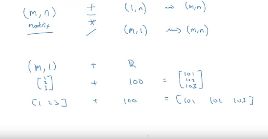
We compute metrics using broadcasting.
Broadcasting is the automatic filling of lists to match matrix shape.
Check the mnist_distance function which is used to do pixel similarity comparison:

{% highlight python %}

def mnist_distance(a,b): return (a-b).abs().mean((-1,-2)) {% endhighlight %}

Why in mnist_distance we are using mean((-1, -2)) is used to find the mean across width and height of the image?
A detailed explanation on this was provided by Srinivas Raman in Week 4 discussion forum:

Since the valid3_tens has a shape of (1010, 28, 28) and the ideal3 will have a shape of (1, 28, 28) with broadcasting, the ideal 3 will be broadcast over the 1st dimension. Now we want the average of the pixel values over the last two dimensions. The last two dimensions which are the height & width of the image are indexed by using the -1 index and -2 index. In python -1 refers to the last element and in this case, the last dim of a tensor and -2 is the 2nd last dim of tensor and so refers to the 28x28 dims of our valid3_tens and valid_tens

Then we found the accuracy of the validation dataset.

For the guest lecture, we had Parul Pandey. Parul had come with an awesome article titled Building a complelling Data Science Portfolio with writing. I will recommend you to watch the Parul Guest lecture from 1:09:30 of the video.

During Parul Pandey’s session, some of my session highlights where:

Parul say’s writing is a personal thing.
Parul doesn’t care about applause. Some of her blogposts has just 83 claps
Work on small small projects, and bring that small projects into life.
Always remember writing takes a lot of time and needs consistency. Yet it has a lot of benefits.
Writing for yourself(growth mindset).

Highlights of the full session can be found by clicking the below video:

Week 4 Discussion forum

defining a numpy array which is used for keeping calories as shown in figure

A = np.array([ [56.0, 0., 4.4, 68.0], [1.2, 104.0, 52.0, 8.0], [1.8, 135.0, 99.0, 0.0]])

calcultes the sum in vertical direction(column wise), so axis = 0

for first element it’s 56+1.2+1.8

cal = A.sum(axis=0) cal {% endhighlight %}

array([ 59. , 239. , 155.4, 76. ])

{% highlight python %} # Divide A which is a 3X4 matrix and divide it by a 1X4 matrix # Note reshape is using broadcasting operation which takes O(1) time 100*A/cal.reshape(1,4) {% endhighlight %}

array([[94.91525424,  0.        ,  2.83140283, 89.47368421],
       [ 2.03389831, 43.51464435, 33.46203346, 10.52631579],
       [ 3.05084746, 56.48535565, 63.70656371,  0.        ]])

General principle of broadcasting

To check more about broadcasting, read NumPy docs as Andrew recommended

Other stuff

I was able to look into the video on Understanding fastai Datablock API
The Tree Classifier web app based on Vue.js + Flask is still a Work in progress. You can check the progress here

Before winding down, Sai Amrit Patnaik has come this week with an excellent initiative:

After interaction with a few members on this fastbook channel who are attending fastbook lectures, there seems to be an interest among many to start an introductory paper reading group and discuss some of the classical papers which laid the foundation of deep learning. The intention is to get started with reading papers and get acquainted and develop a habit of reading papers while learning the basics more comprehensively and without worrying much about technicalities in the latest papers.

Thank you everyone for reading 🙏. Please feel free to share your suggestions, questions, queries through the comments below..

Recap of Week 4

Now let me share some of my learnings over the week:

defining a numpy array which is used for keeping calories as shown in figure

calcultes the sum in vertical direction(column wise), so axis = 0

for first element it’s 56+1.2+1.8